EO/IR (Electro Optical / Infrared) systems and long range thermal cameras cover a wide range of distinct technologies based on the targets and mission to be accomplished.

Target phenomenology often dominates the choice of spectral band. For example, missile launch detection depends on the very hot missile exhaust, which produces significant radiation in the ultraviolet (UV) spectral region. The band choice is also influenced by the vagaries of atmospheric transmission and scattering

EO/IR missions divide roughly into dealing with point targets and extended fully imaged targets. For point targets, the challenge is to extract the target from a complex and cluttered background. For fully imaged targets (images of tanks, for example), the contrast between target and background is a critical parameter. The ability to detect dim targets, either point or extended, is a measure of the system’s sensitivity. The resolution of a sensor is a measure of its ability to determine fine detail. Measures of resolution depend on the precise task. Use of eye-chart-like calibration targets is common in DoD applications. EO/IR sensors may be divided into scanning sensors, which use a limited number of detectors to scan across the scene, and staring sensors, which use large numbers of detectors in rectangular arrays.

Non-Imaging EO/IR Systems

Non-imaging point target EO/IR systems focus on the task of detecting targets at long range. For these applications, details of the target are irrelevant; for example, for IR sensors, only the total energy emitted matters, not the precise temperature and size of the target separately. The available energy can vary over many orders of magnitude, from the engine of a small UAV to an intercontinental ballistic missile (ICBM) launch.

Comparison of the available energy at the sensor to the noise level of the sensor provides the central metric of sensor performance, the noise equivalent irradiance or NEI. The problem of extracting the target from background clutter is addressed in two basic ways: through the choice of sensor band and algorithms. For missile launch detection, for example, one may use the “solar blind” UV band.

The transmission in this band is very poor, and the general background is reduced to a level of near zero. However, the very bright missile signature is strong enough to still provide a useable signal. Algorithms for separating a point target from a structured background are a continuing source of improvement in performance, but their complexity may make their evaluation challenging.

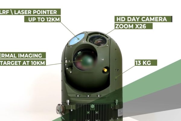
THERMAL IMAGING FLIR PTZ CAMERA SELECTION:

M5 LONG RANGE PTZ THERMAL IMAGING FLIR CAMERA

M7 LONG RANGE PTZ THERMAL IMAGING FLIR CAMERA

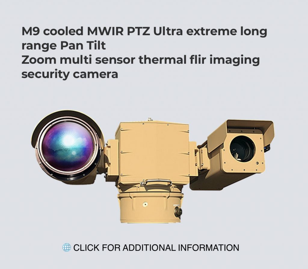
M9 LONG RANGE PTZ MULTI SENSOR THERMAL IMAGING FLIR CAMERA

M11 LONG RANGE PTZ TJERMAL IMAGING FLIR SECURITY CAMERA 

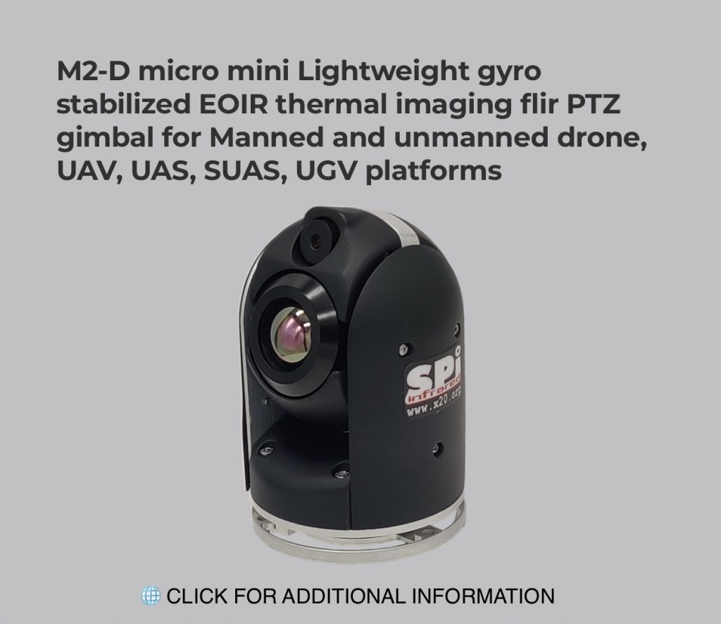
M2D LONG RANGE DRONE GYRO STABILIZED DRONE THERMAL IMAGING FLIR OTZ CAMERA GIMBAL FOR UAS UGV UAV AND SUAS

M1D VEHICLE MOBILE MARINE ROOF OR STATIONARY MOUNTED LONG RANGE PTZ THERMAL IMAGING FLIR TURRET CAMERA SYSTEM

The effectiveness of imaging systems can be degraded by many factors, including limited contrast and luminance, the presence of noise, and blurring due to fundamental physical effects. As a mathematical description of image blur, the MTF can be broken down into each component of the sensing, such as optics, detector, atmosphere, and display. This provides insight into the sources and magnitude of image degradation.

There are many ways to evaluate and describe the quality of an image, the use of which is determined by details of the application. Two examples have a broad application and a long history.

1. The Army Night Vision and Electronic Sensors Directorate (NVESD) maintains models for predicting image quality based on the targeting task performance (TTP) metric.1 This provides a rule-of-thumb for the number of bar pairs required on target to have a 50-percent probability of detecting, recognizing, or identifying the target.
2. The strategic intelligence community uses the National Imagery Interpretability Rating Scale (NIIRS) to evaluate the quality of still imagery. NIIRS is a qualitative scale, running from 0 to 9. Tables are published associating rating levels with tasks for EO, IR, synthetic aperture radar (SAR), civil imagery, multispectral imagery, and video. NIIRS can be estimated by the General Image Quality Equation (GIQE), an empirical model that has been designed to predict NIIRS from sensor system characteristics.

Each of these approaches represents a balance between two of the fundamental limits to any EO sensor: the resolution (how small) and the sensitivity (how dim) – that is, how small an object or feature can be usefully seen and how low can the signal be before it is overwhelmed by the noise. Figure ES-1 shows a comparison of a noise- limited case and a resolution-limited case.

1 The TTP metric is the successor of the Johnson criteria. See page 30 for additional discussion.

In modern digital sensors, these classical factors have been joined by a third, the sampling or pixelation of the sensor, as shown in Figure ES-2.

ES-2. Sampling Limited Image

The design of a sensor is a tradeoff between these three factors, placed in the context of characteristics of the target and environment. While in a balanced design, each of the factors needs to be evaluated. For any given sensor and state of the technology employed, it may be the case that the sensor is signal-to-noise limited; in this case, the S/N ratio is the single-most important parameter and rules-of-thumb may be developed to focus on S/N for the target and environment. In other cases, the sensor is resolution limited, and the characterization of the optics (the MTF) is the most important; an ideal sensor is said to be diffraction-limited, able to respond to spatial frequencies up to the diffraction limit, λ/D, where λ is the wavelength at which the sensor operates and D is the diameter of the optics. For these cases, rules-of-thumb may be developed that focus on the optical system. For sensors that are limited by the pixelation, the “Nyquist limit” is determined by the separation between detectors, S; the highest spatial frequency that can be correctly measured by the sensor is 1/2S. In these cases the Nyquist frequency may be an appropriate rule-of-thumb.

These trades can be followed in the history of personal cameras from the film era to the most modern Nikon or Canon. In the film era, the user could trade between sensitivity and resolution by changing the film used: so-called fast film (TRI-X) was sensitive but had a coarse grain size, limiting the resolution. It was useful for pictures in dim light or when high shutter speeds to photograph moving subjects were needed. In brighter light or for slowly moving objects the photographer might choose a slow film (PAN-X) that had a fine grain size but was not very sensitive. On top of this choice, the photographer could choose lenses with different f-numbers (to change sensitivity), different focal lengths (to change resolution), and different prices (to improve MTF).

In the last 2 decades, digital cameras have replaced film cameras in many applications. The earliest digital cameras were limited both by sensitivity (detectors were noisy) and by sampling. In consumer terms, the sampling resolution was specified by the

number of pixels; early cameras were 1 megapixel, about 1,000 by 1,000 detectors replacing the film. The need for relatively large detectors (10-20 μm) was driven by lack of detector sensitivity; the resulting reduction in resolution compared to the better films that had film grains of 2-3 μm was a consequence of this, rather than a technological limit to producing smaller detectors. As detector technology evolved, the noise in each detector was reduced (improving S/N and allowing dimmer light or faster motion) and the number of pixels was increased. Today, personal cameras can have 36 megapixels or more and begin to rival the finest grain films for resolution with detectors of 4 μm or smaller. The best personal cameras began as sensitivity and sampling limited; but as those barriers were overcome, they have returned to being resolution limited as determined by the quality of the optics. As these changes have taken place, the simple rules-of-thumb that characterize the camera have also changed.

The same three elements are present in all EO systems, but there is no unique balance point between them. This is determined by the state of technology but also the mission the sensor is trying to accomplish. Personal cameras emphasize images of people at close to moderate ranges; the signal is determined by reflected light, the noise by the technology of the detectors. Missile launch detection systems are looking for extremely bright points of light in a cluttered background. Infrared systems depend on the self-emission of the target (hot engines on aircraft and tanks) and are often limited by the environment (the transmission of the signal through the air). No matter what the sensor is, the evaluation of the sensor system involves characterizing it with the three metrics of noise, resolution, and sampling.

Tracking

EO/IR sensor systems are often paired with a tracker. Examples of point target trackers include systems to track missile launches and infrared search and track systems, both discussed above. Many different algorithms are used to implement point trackers. Although different, they all involve the same basic steps: track initiation, data association, track smoothing, and track maintenance. Conversely, image-based trackers are used to track mobile objects on the ground [e.g., intelligence, surveillance, and reconnaissance (ISR) missions] or for aim point selection. Usually with image-based trackers, the target is initially located by a human operator viewing a display. After the target is acquired, a feedback control loop (track loop) continuously adjusts the gimbal to keep the target in the center of the sensor’s field of view. Common image-based tracker algorithms include edge detection, centroid tracking, area correlation tracking, moving target indicators (MTI), multi-mode trackers, and feature-based algorithms.

Latest Trends in EO/IR System Development

Driven by missions such as Persistent Surveillance, an important recent trend in EO/IR sensors is the development of large-area, high-resolution cameras. For sensors operating in the visible band, this is simpler than for those operating in the mid-

wavelength infrared (MWIR) or long-wavelength infrared (LWIR) bands. In the visible band, silicon can be used for both sensing material and for readout electronics. This eliminates issues such as potential thermal mismatch between the two. For EO systems, it is also possible to group individual cameras together and then combine separate images into one. The current state of the art in MWIR focal plane arrays (FPAs) is roughly 4,000 by 4,000 detectors; for LWIR FPAs, it is closer to 2,000 by 2,000. The ARGUS sensor being developed by DARPA has 1.8 gigapixels. To reduce the amount of thermally generated noise in LWIR FPAs, these cameras operate at low temperatures. The required cryogenic equipment has important Size, Weight, and Power (SWaP) implications at the system level and can affect system reliability. To address this need, considerable effort has gone into development of uncooled sensors. Another recent development is the use of so-called III-V superlattices that use alternating layers such as aluminum gallium arsenide and gallium arsenide (AlGaAs/GaAs) and that allow one to change the device’s spectral response by changing individual layer thicknesses. The short-wavelength infrared (SWIR) band extends from 1.0 μm to 3.0 μm. This radiation, often referred to as “airglow” or “nightglow,” is non-thermal radiation emitted by the Earth’s atmosphere. Military applications of SWIR include low-light/night-vision imaging, detection of laser designators, covert laser illumination, laser-gated imaging, threat-warning detection, ISR, and covert tagging. Hyperspectral imaging allows one to simultaneously gather both spatial and spectroscopic information for more accurate segmentation and classification of an image.

Aliasing

Aliasing is an almost inescapable feature of staring focal plane array sensors. Aliasing refers to the artifacts associated with sampling systems. They can range from Moiré patterns2 to ambiguously interpreted images of objects with complicated patterns of light and dark. The presence of aliasing in a system gives rise to a general rule based on the Nyquist frequency, which identifies the resolution of a system with the size of a sample (or pixel) on the target. This underrates the importance of other determiners of resolution such as the MTF. Performance may be better or worse than that suggested by Nyquist, depending on the task. The combination of MTF and aliasing can lead to some unintuitive tradeoffs. For example, poorer MTF may actually improve performance in some tasks if aliasing is a significant problem. For imaging systems with aliasing, the display of the sensor information becomes important, especially if the image is zoomed so that one display pixel is used to represent a single sensor sample value. An improper reconstruction of the sensor data can degrade performance. For all aliased systems, an understanding of the reconstruction algorithm is an important aspect of any system including a human operator.

2 Moiré patterns are interference patterns that are often the result of digital imaging artifacts. See page 59 for additional discussion.

Issues in Bayer Color Cameras

The use of Bayer pattern color cameras in imaging systems to reduce cost and data rate requirements may introduce additional dependence on algorithmic choices. In contrast to full color cameras, a Bayer camera does not have a color detector for all 3 colors (red, green, blue) at each location (a 12 “megapixel” Bayer sensor has 6 million green, 3 million red, and 3 million blue detectors). An algorithm is used to interpolate the missing values to produce a complete three-color image. This color aliasing is more severe than the aliasing intrinsic to any staring focal plane. Fortunately, in the natural world, color information is usually relatively immune to aliasing effects. However, a large number of different algorithms of varying complexity may be employed by a sensor manufacturer. Depending on the tasks to be performed and the details of the image, the algorithm may induce new artifacts that complicate system evaluation. Ideally, the user could be given some control over the interpolation algorithm to match it to the task.

A Tutorial on Electro-Optical/Infrared (EO/IR) Theory and Systems

The most basic division in EO/IR sensors is between point and extended targets. A point target is one that is small enough, compared to the resolution capabilities of the sensor, to appear as a single point. The defining characteristic of an extended target is the presence of internal detail. Rather than detecting a point, the sensor presents an image of the target. The distinction between point and imaging targets is not the same as between non-imaging and imaging sensors. One can imagine a point target mission that scans the sky looking for a bright spot without ever forming an image (the original Sidewinder air-to-air missile seeker would be such as system); however, some imaging sensors form an image of the sky and then look for bright spots within the image.

Infrared search and track (IRST) systems represent a class of systems for which the targets remain point targets. The term primarily refers to IR sensors dedicated to detecting aircraft at long range. Aircraft are typically hotter than the sky or cloud background against which they are seen and appear as a bright point. Although originally conceived as an air-to-air aircraft finder or a ship-to-air missile finder (to detect anti-ship cruise missiles), the same approach has applications for homeland security and anti- unmanned aerial vehicle (UAV) search. Another class of systems is missile-launch detection systems. In this case, the launch is signaled with a very hot flash that can be

detected. In this case, the background is likely to be the ground rather than the sky for IRST systems; this affects the algorithms used to extract the target and even the band (wavelength) of the EO/IR sensor.

The extended target applications include intelligence, surveillance, and reconnaissance (ISR) systems providing long-term imaging of the ground, usually from a vertical perspective (e.g., surveillance satellites, UAV), and target acquisition systems in tactical systems [night vision goggles, tank forward-looking infrared (FLIR) systems], typically a more nearly horizontal view.

The definition of each of the terms mentioned above will be developed over the course of this paper.

It may be surprising to see film discussed in the 21st century; however, in some ways, film remains unsurpassed.

Developed in the early 1960s, the U-2’s Optical Bar Camera (OBC) gave the spy plane an edge that has yet to be matched by its prospective successor: the Global Hawk unmanned aircraft. The film camera, which is mounted in a bay behind the aircraft’s cockpit, captures high-resolution panoramic images covering an area 140 degrees across.

The OBC gets its name from its slit assembly, which forms the camera’s bar. Unlike a conventional camera, in which an aperture opens and closes to allow light to expose the film (or, in the case of a digital camera, a charge coupled device chip), the slit exposes a roll of film mounted on a 3-foot-diameter rotating spindle. The entire lens assembly, with a 30-inch lens, rotates around the longitudinal axis of the aircraft to provide a field of view that extends 70 degrees to either side of the aircraft’s flight path.

The OBC carries a roll of film measuring some two miles in length and weighs around 100 pounds. Each frame is 63 inches long by 5 inches wide.

A. Basics

EO/IR systems are often plagued by the difficulty of providing precise predications of performance: in EO/IR, the answer is “It depends.”

The majority of EO/IR systems (laser systems are the conspicuous exception, but searchlights are still used as well, and night vision goggles can be used with artificial illumination) are passive; that is, they are dependent on the illumination of the target by sunlight or moonlight (even sky shine) or the target’s own emission of light. This is in contrast to radar systems that provide their own illumination. In addition, the EO/IR photons travel through a hostile medium, the atmosphere, which can refract, absorb, or scatter them. EO/IR is, in general, sensitive to the environment. Also, the target’s characteristics can be quite important and variable, depending on the target temperature and even the paint used on the target. This variability poses a problem to the designer, tester, and operator.

The designer has more control over the sensor’s design parameters, datalinks used to transfer information, and displays on which, for imaging sensors, the scenes are presented to the human operator.

Electro-optical/ Infrared Systems

• EO/IR systems cover the range from UV through visible and IR. 0.38 -0.75 m
• The wide range of EO/IR systems share some similarities:
  • –  Lenses and mirrors rather than antennas
  • –  Dependence on the environment
• Although film systems remain in the inventory and are still preferred for some missions, new EO/IR systems will be digital.
• The band chosen reflects the phenomenology of the target. Image Source:

LWIR: emitted radiation

D. G. Dawes and D. Turner, “Some Like It Hot,” Photonics Spectra, December 2008.

SWIR: reflected radiation

The category of EO/IR sensors extends from the ultraviolet at a wavelength of 0.25 micrometers (μm) (which can be useful for very hot missile launch detection applications) through the visible region to the infrared region (wavelengths up to 14 μm or even greater). The design wavelength band is determined by the expected targets and mission.

As noted in the chart, the choice of wavelength is connected to the balance of emitted versus reflected light. One obvious difference is that human operators are accustomed to how objects appear in reflected visible light. The short wave IR, which almost entirely depends on reflected light, produces images that are very like visible images; mid-wave IR, less so; and for long-wave IR, the images seem unnatural in some aspects.

Emitted radiance (L) of blackbody3 with temperature T and emissivity ε between λ1

and λ2 is given by: 𝐿photons = �

2𝜀(λ) 2𝑐 𝑒 1 λ 4 h𝑐/𝑘𝑇λ

− 1 𝑑λ
2h𝑐1 1 h𝑐

2 λ 𝑑λ ≈ 𝐿 h𝑐/𝑘𝑇λ

𝐿 = �λ 𝜀(λ)
watts 2 λ𝑒 −1 photonsλ

λ1 λ5

sensor

For most modern EO/IR sensors, the photon representation is the more appropriate because the detectors are essentially photon counters. However, very early IR systems and some modern uncooled systems are bolometers, measuring the energy of the signal rather than the number of photons. For these systems, the radiance in terms of watts is the more useful. The terminology can be quite confusing and care must be taken to keep the units straight.

3 A blackbody is an idealized physical body that absorbs all incident electromagnetic radiation, regardless of frequency of angle of incidence. A blackbody at constant temperature emits electromagnetic radiation called blackbody radiation. The radiation is emitted according to Plank’s law, meaning that it has a spectrum that is determined by the temperature alone and not by the body’s shape or composition.

(wiki)

The complicated structure of the atmospheric transmission curves reflects the fact that the atmosphere is a mixture of different molecules with each species having its own set of absorption and emission lines. Because it is a mixture, the curves will depend on, for example, the absolute humidity (the water content of the air). Pollutants such as ozone or discharges from factories can be relevant, as can aerosols suspended in the air, including water (ordinary haze and fog), sand, dirt, and smoke.

Although it is common to assume a simple exponential decay of transmission with range (so-called Beer’s Law), it is never safe to do so without checking the more elaborate calculations involving individual absorption lines, rather than averages over bandwidth ranges. The dependence of EO/IR on transmission is the primary factor that makes the predicting and testing of EO/IR systems challenging.

There are many different definitions of resolution, each of which is connected to a specific task. For example, mathematically, the Rayleigh criterion requires the signal from one point (star) to fall to zero. Two stars are resolved when one star is located at the first zero point of the other. The Sparrow criterion for stars only requires that there be a dip in the brightness of the combined image; so two stars may be resolved on the Sparrow criterion, but not on the Rayleigh criterion.

Although the use of a calibration target with bar groups of different sizes is relatively standard, the results of a test will depend on the number of bars in a bar group, the aspect ratio of the bars, and the instructions to the test subject explaining the criterion for declaring a bar group resolved.

Historically, the difficulty in manufacturing large square or rectangular focal plane arrays has meant that many sensors used scanning designs. There is a general migration from scanning to staring sensors. However, in some cases, a line-scanner may still provide the best solution. For example, if one wants a number of different colors or bands, a line-scanner can simply add more rows of detectors for the additional colors. Although some technologies provide, for example, a two-color IR array, achieving four or more colors requires a complicated design with multiple staring arrays. For applications requiring a wide field of view, it may be easier to create a 10,000-element linear array for a line-scanner than a 1-million element detector staring array.

Basics Summary

• EO/IR systems cover a wide range of distinct technologies based on the targets and the mission to be accomplished. The target phenomenology may dominate the choice of spectral band. For example, missile launch detection depends on the very hot missile exhaust, which produces the majority of radiation in the UV. The band choice is also influenced by the vagaries of the atmosphere (transmission and scattering).
• EO/IR missions divide roughly into dealing with point targets and fully imaged targets. For point targets, the challenge is to extract the target from a complex clutter background. For fully imaged targets (images of tanks, for example), the contrast between the target and the background is a central parameter. The ability to detect dim targets, either point or imaged, is a measure of the system’s sensitivity.
• The resolution of a sensor is a measure of its ability to determine fine detail. Measures of resolution depend on the precise task. The use of eye-chart-like calibration targets is common in DoD applications.
• The technology used in EO/IR sensors may be divided into scanning sensors, using a limited number of detectors that scan across the scene, and staring sensors, using large numbers of detectors in rectangular arrays.

B. Non-Imaging EO/IR Systems

Non-Imaging EO/IR systems

• Non-imaging systems refer to unresolved or point targets.
  • –  The simplest example of a point target is a star: in the sensor, a star produces an image that is called the point target response, impulse response, or blur circle. It may cover more than one detector element.
  • –  An unresolved target is any object that produces an image in the sensor comparable to that of a star: there is no internal detail.
  • –  For a resolved target, some amount of internal detail can be recovered.
  • –  The rule of thumb is that a target is resolved if the sensor can put multiple detector fields of view on the target; unresolved if the target is entirely contained within one instantaneous field of view (IFOV).
  • –  IFOV = detector size (d) / focal length (fl)
• For a point target, the only signature characteristic is the amount of energy emitted in a specified direction or radiant intensity measured in watts/ster or spectrally (as a function of wavelength) watts/ster/μm– Radiant intensity ≈ Area target * radiance = AT * LT– LT is the power per unit solid angle per unit projected source area.– Radiant intensities for small aircraft (UAV) are the range of 0.05 watts/ster in MWIR and 0.25 watts/ster in LWIR.

– For ballistic missiles the signatures are much higher, megawatts/ster.
• Radiant intensity of the target is compared to that of the background:

radiant intensity contrast ≈ A *( L – L ) T T Background

Instead of using watts/ster,4 it is sometimes more convenient to describe the photon flux, photons/sec/ster. The common unit for IR systems is the watt, but, for visible systems, photons/sec is often employed.

The instantaneous field of view (IFOV) is a fundamental sensor parameter. At range R, a single IFOV covers a distance D = IFOV*R. As an example, detectors for visible digital cameras (Nikon, Canon) are about 10 μm in size. With a 100-mm lens the IFOV = (10*10-6)/(100*10-3) = 10-4. At a range of 1,000 meters, the IFOV covers 10 cm. If the target were 1 meter x 1 meter, we might say there were 10 x 10 = 100 IFOVs on target; this is usually replaced with the sloppier phrase, 100 pixels on target.

4 The steradian is a unit of solid angle. It is used to quantify two-dimensional angular spans in three- dimensional space, analogously to how the radian quantifies angles in a plane. (wiki)

Non-Imaging Applications

• Air-to-air (Sidewinder) — First Sidewinders had a single detector behind a rotating reticle. Modern air-to-air missiles use focal plane arrays but, at long range, the target is a point target.
• IRST (Infrared Search and Track)
  • –  Air-to-Air — Permits passive operation of aircraft. Limited by cloud clutterbackground.
  • –  Surface (Sea)-to-Air — Radar detection of sea-skimming cruise missiles may be adversely affected by environment effects. IR has different environmental problems and may provide a supplement to radar.
  • –  Surface (Ground)-to-Air — For identification and tracking of small aircraft (UAV) EO/IR may offer advantages in resolution.
• Missile launch detection
  • –  Usually based on missile plume detection
  • –  Tactical warning systems
  • –  Strategic warning (DSP/SBIRS)The reticle was an engineering marvel. A reticle rotating disk has a pattern of transparent and opaque sectors. For a point target, the rotating pattern provided a blinking signal that could be distinguished from the background (clouds or sky), which did not vary as much. Further processing of the shape of the blink actually provided sufficient information to guide the missile to the target, directing it to maneuver up, down, left, or right.However, the problems of clutter rejection and dependence on atmospheric conditions are barriers to IRST use.

For any sensor to be evaluated, the first step in understanding the expected performance is to understand the signal produced by the target. The signal provided by a point target is particularly easy to understand. The example introduces several generally useful concepts. The radiant intensity contrast is a characteristic of the target at the source; using the photon (rather than watt) description, it represents the number of additional photons/sec/ster being radiated (or reflected) because the target is there.

The analysis of the signal given on the preceding chart implicitly assumed that all the photons from the target were easily counted. This would be the case if all the photons landed on a single detector. However, even if the point target image (or “blur circle”) is small compared to the detector, the spot may land on the boundary between detectors so a fraction of the signal falls on one detector and another fraction on another. In the worst case, the signal would be reduced to 1⁄4 of the nominal value, divided among four detectors. The detection algorithms used in this limit may look at the detector output of several detectors to increase the detection range.

In the other limit, the size of the blur circle may be large compared to the detector. Surprisingly, this can be an advantage in some point target applications if the expected signal level is high enough. For a tiny blur circle, one can only say that the target is located somewhere in the field of view of that detector. If the blur circle covers several detectors, a model of how the signal should vary from detector to detector can allow an estimate of the location of the target to a fraction of an IFOV. This is also called “sub- pixel localization.”

In most applications, the detection algorithms are as important in determining performance as the sensitivity of the detectors and IFOV. The point targets may be seen against a complicated clutter background; simply looking for a hot spot may produce an unacceptable number of false alarms.

In EO/IR sensors, estimating and characterizing noise and clutter is a vital element for understanding system performance. The use of a “clutter-noise” term is a common first order attempt to incorporate the clutter into performance estimates. However, since the scene is processed through a series of algorithms (which, in some applications may be quite complex), the effect of clutter has to be considered after the algorithms are run, not before. Estimates of performance require substantial testing or laboratory testing with scene simulators, the use of which must be examined carefully to ensure that the simulator presents the relevant features of the clutter. What sort of clutter is relevant depends on the algorithms!

To be more precise, the Lbackground should include not only the background radiation at the target but also the so-called “path radiance,” radiation emitted between target and sensor by the atmosphere.

𝐿 = 𝐿 (𝐼𝑜 𝑜𝐼𝐼𝑆𝑒𝑜) + 𝑝𝐼𝑜h 𝐼𝐼𝑑𝐼𝐼𝑜𝑐𝑒 (𝑁𝑒𝑜𝑏𝑒𝑒𝑜 𝑜𝐼𝐼𝑆𝑒𝑜 𝐼𝑜𝑑 𝑜𝑒𝑜𝑜𝑜𝐼) 𝑡𝑜𝑡𝑎𝑙 𝑏𝑎𝑐𝑘𝑔𝑟𝑜𝑢𝑛𝑑

Noise equivalent irradiance (NEI) is an example of a number of similar figures of merit. For example, the irradiance of a target depends on the difference in the radiance of the target and background. For a system that utilizes the target’s temperature and its emitted radiation, the radiance difference can be considered to be attributable to the difference in temperature between target and background. If the temperature difference is relatively small, the irradiance will be proportional to the temperature difference, ∆T.

EO/IR systems are often dominated by environmental effects. Normally one chooses a band with good transmission, but, with good transmission, one can see all the clutter as well as the target. By choosing a band with poor transmission, very bright targets can still be seen but the clutter becomes invisible. If this trick isn’t used, the targets must be separated from the background by means of detection algorithms. Any detection algorithm is associated with both a probability of detection (Pd) and a false alarm rate (FAR). Typically, internal parameters, or “thresholds” in the algorithm, permit the designer to trade off probability of detection and false alarm rate. The curve relating the two is termed the “ROC curve”; ROC is an acronym of ancient origin for “receiver operating characteristic.” Testing and evaluating the detection algorithm is difficult because of the wide range of potential clutter backgrounds. Some systems may employ scene simulators that use models of background clutter to produce a wide range of scenes purported to span the circumstances of the real system in the real environment.

Point Target Summary

• Non-imaging, point target EO/IR systems focus on the task of detecting targets at long ranges. For these applications, the details of the target are irrelevant; for example, for IR sensors, only the total energy emitted matters, not the precise temperature and size of the target separately. The energy available can vary over many orders of magnitude, from the engine of a small UAV to an intercontinental ballistic missile (ICBM) launch.
• Comparison of the available energy at the sensor to the noise level of the sensor provides the central metric of sensor performance, the noise equivalent irradiance or NEI.
• The problem of extracting the target from the background clutter is addressed in two basic ways: through the choice of sensor band and algorithms. For missile launch detection, for example, one may use the “solar blind” UV band. The transmission in this band is very poor and the general background is reduced to a level of near invisibility. However, the very bright missile signature is strong enough to still provide a useable signal. Algorithms for separating the point target from the structured background are a continuing source of improvement in performance, but their complexity may make the evaluation challenging.

C. Imaging EO/IR Systems

The choice of optics and detector affect the magnification provided and image clarity. Image quality includes measures of:

• Contrast – Degree of difference between lightest and darkest portions of image
• Luminance – Brightness of image
• Noise – Random signal from sources outside the image itself
• Sampling – Digitization due to binning of signal into pixels
• Blur – Smearing of image due to diffraction and/or imperfect focus (e.g., due to jitter).

Classical MTF measurements in the laboratory are made more complicated by aliasing effects. One approach to overcome aliasing is to displace the image of the calibration target to provide different sample phasing (see p.60). For examples of other efforts made to work around the sampling artifacts, see Research Technology Organization Technical Report 75(II), Experimental Assessment Parameters and Procedures for Characterization of Advanced Thermal Imagers.

Aliasing refers to the inability to correctly represent spatial frequencies higher than the Nyquist frequency of a digital system. This will be discussed in detail in Section F.

This chart provides an initial discussion of why modern staring systems are typically aliased. For a staring array of square detectors, the detector MTF is given by

𝑀𝑇𝑀𝑑𝑒𝑡(𝑜) = 𝑜𝐼𝑜𝑐(𝜋𝑜𝜋) =

𝑜𝐼𝑜(𝜋𝑜𝑑) 𝜋𝑜𝑑

The detector MTF therefore extends to all frequencies. The first zero of the detector MTF is at f = 1/d; subsequent zeros are at multiples of that frequency, f = m/Wd m= 1, 2, 3….

However, the Nyquist frequency for such an array is fNyquist = 1/2d. Even if the frequencies beyond the first zero of the MTF are ignored (because of their diminishing amplitudes), the system is under-sampled by a factor of 2.

This may be modified by the consideration of the optics MTF, represented here by straight lines (correct for a square not circular lens!). If the blur circle of the detector (first zero) fits inside the detector, the optics MTF extends to 2/d (and is zero for high frequencies). This would mean being four times under-sampled (maximum frequency 4 x Nyquist). Degrading the optics until the blur occupies four detectors leads to the “matched optics” condition for which the optics MTF zero coincides with the first detector zero. Only if the blur occupies 16 detectors does the optics MTF zero match the Nyquist limit.

As shown in the preceding examples and to be developed further, this elimination of all potential aliasing reduces the system MTF (contrast) significantly. Most design trades permit some aliasing in order to preserve useable image contrast.

In classical noise equivalent temperature difference (NETD), the signal was compared to a measure of the temporal noise of the system (as measured through a standard electronic filter). In modern staring focal plane arrays, other noise sources must be considered. For example, each detector in the array will generally have a different response; this is called detector non-uniformity. Although an effort is made to provide non-uniformity correction, any residual non-uniformity represents a static spatial pattern noise. In addition, individual detectors may be uncorrectable, noisy, or dead.

The NVESD has introduced a three dimensional (3D) noise model to describe noise components in the temporal and two spatial dimensions.

One approach taken by NVESD5 and others to represent the effect of aliasing on the MTF is to represent the MTF of the sampled system by squeezing (scaling) the MTF of the corresponding unsampled system.

The factor R = 1 – k SR, where SR is a metric representing the spurious response. The value of the constant k may vary with task (detection, recognition, identification) and different forms of the SR metric have been used. H(f) is the Fourier transform of the reconstruction function used. See Section G on aliasing.

Another approach is to treat aliasing as a noise term.6

An extension of the MRT task, the Minimum Temperature Difference Perceived (MTDP) has been introduced in Germany. This provides an extension beyond Nyquist.

5. 5  Driggers, Vollmerhausen, and O’Kane, SPIE, Vol. 3701, pp. 61-73, 1999.
6. 6  Vollmerhausen, Driggers and Wilson, JOSA-A, Vol 25, pp. 2055-2065, 2008.

Performance metrics can be affected even by simple gain and level adjustments.

Contrast = (Signal – Background)/Background = (S-B)/B

is unaffected by a change of scale (gain) but is changed dramatically with a level shift:

Contrast = ((S-L) – (B-L))/(B-L)= (S-B)/(B-L). Signal-to-noise (SNR) = (S-B)/Noise

is unaffected by gain or level as long as values are not truncated or saturated. In some applications, gain and level may not be under user control.

In 1957 and 1958, John Johnson at the Army Night Vision Laboratory developed a series of experiments to analyze the ability of observers to perform visual tasks, such as detection, recognition, and identification. He came up with general rules for the number of bar pairs required on target to have a 50-percent probability of performing each of these tasks. Over time, this approach has evolved to account for the increasing sophistication of today’s EO/IR sensors. The Army Night Vision and Electronic Sensors Directorate (NVESD) maintains models for predicting image quality based on the targeting task performance (TTP) metric, the successor to the Johnson criteria. Very recently, the visible and IR models, known as Solid State Camera and Image Processing (SSCamIP) and Night Vision Thermal and Image Processing (NVThermIP), respectively, have been combined into one software package, known as the Night Vision Integrated Performance Model (NV-IPM).

As an example, the Johnson criteria can be applied to determine the number of pixels in an image required to detect, recognize, and identify a human subject. The calculations shown here are illustrated by the images on the chart below.

The eye contrast threshold function has been measured by repeated experimentation on a large group of observers. The experiment entails showing two fields to the observers. One field contains alternating black and white bars, and the second is constant gray of the same total luminance. The observers are asked to identify which of the images contains the alternating bars. This experiment is repeated as the contrast of the bar pattern is changed, while keeping the total luminance constant. The contrast at which 75 percent of the observers correctly identify the bar pattern is considered the threshold for that level of luminance. (The threshold is set at 75 percent because in a two- alternative forced choice experiment such as the one described here, the right answer will be selected 50 percent of the time simply by chance.) By conducting this experiment at varying spatial frequencies (i.e., bar spacings), one of the curves shown above can be measured. Differing levels of luminance give rise to the series of curves shown above.

An example of the experiment described in the previous chart is displayed here.

The zero range target contrast is a measure of the inherent contrast between the target and the background, independent of the distance between the target and sensor. In the visible, the contrast at each wavelength is integrated over the visible portion of the electromagnetic spectrum to determine the zero range target contrast. In the infrared, the contrast is due to the difference in thermal emission between target and background. The zero-range contrast is then attenuated by atmospheric effects, which can be treated as homogeneous or modeled in a complex computer program, such as MODTRAN (MODerate resolution atmospheric TRANsmission). The apparent target contrast is also degraded by scattering of light into the path between target and sensor.

The Army has introduced the concept of sky-to-ground ratio (SGR) to account for the scattering of light into the path between target and sensor. Values of SGR typically range from 1.4 in clear conditions with low relatively humidity to well over 10 when the path radiance is high, due to multiple scattering events, as would be encountered when the sun is shining directly on the target-sensor path or in a forest under overcast conditions.

The strategic intelligence community uses the National Imagery Interpretability Rating Scale (NIIRS) to evaluate the quality of still imagery. NIIRS is a qualitative scale, running from 0 to 9, with guidance for imagery analysts provided in the form of a table of example operations that could be performed at various NIIRS values. The table for visible NIIRS values is provided on the following chart. There are also tables for IR NIIRS, synthetic aperture radar (SAR) NIIRS, civil imagery NIIRS, multi-spectral NIIRS, and video NIIRS.

NIIRS can be estimated with the General Image Quality Equation (GIQE), an empirical model that has been designed to predict NIIRS from sensor system characteristics. In the visible, the GIQE takes the form

NIIRS = 10.251 – a log GSD + b log RER – 0.656 H – 0.344 (G/SNR)

where GSD is the ground sample distance RER is the relative edge response H is the overshoot,
G is the gain,

SNR is the signal-to-noise ratio,
a = 3.16
b = 2.817 for RER < 0.9 and a = 3.32, b = 1.559 for RER ≥ 0.9.

The only change to the GIQE in the IR is that the constant term is 10.751, rather than 10.251. The GSD, RER, and overshoot will be defined and discussed in subsequent charts.

Ground sample distance (GSD) is the dominant term in the GIQE and ultimately provides an upper limit to the image quality, since all information in the area defined by the horizontal and vertical GSDs is incorporated into a single pixel. The GSD is defined by

where PP is the pixel pitch x is the slant range

FL is the focal length

GSD = ((PP * x)/FL)/cos θ

θ is the look angle, measured between nadir and the sight line.
For non-square pixels, the vertical and horizontal GSDs differ and are specified separately.

The blurring of the original image as adjacent pixels are averaged together is evident in comparing the image in the upper left quadrant to that in the upper right quadrant and finally to that in the lower left of the figure.

The relative edge response is a measure of blur and is defined to be equal to the difference in the normalized edge response 0.5 pixels to either side of an edge. In a perfect image where a completely black area is adjacent to a completely white area, the pixel on one side of the edge has a luminance of one whereas the pixel on the other side has a luminance of zero. In reality, blurring of the black and white portions occurs in the vicinity of the edge. Edge analysis is conducted on real images to ascertain values of relative edge response (RER) for actual sensors.

Overshoot is due to excessive use of a digital process to sharpen imagery at edges (MTF compensation). It is defined to be the value of the peak normalized edge response in the region 1-3 pixels from the edge, unless the edge is monotonically increasing in that range, in which case, it is defined as the edge response at 1.25 pixels from the edge. This term partially offsets the improvement in NIIRS that a really sharp edge response provides.

Imaging EO/IR Systems Summary

• The effectiveness of imaging systems can be degraded by many factors, including limited contrast and luminance, the presence of noise, and blurring due to fundamental physical effects.
• MTF is a mathematical description of image blur and can be broken into each component of the sensing, such as optics, detector, atmosphere, and display, providing insight into the sources and magnitude of image degradation.
• The Army NVESD maintains models for predicting image quality based on the TTP metric, the successor to the Johnson criteria, rules of thumb for the number of bar pairs required on target to have a 50-percent probability of detecting, recognizing, or identifying the target.
• The strategic intelligence community uses NIIRS to evaluate the quality of still imagery.
  • –  NIIRS is a qualitative scale, running from 0 to 9.
  • –  Tables are published associating rating levels with tasks for EO, IR, SAR, civil imagery, multi-spectral, and video.
  • –  NIIRS can be estimated by the GIQE, an empirical model that has been designed to predict NIIRS from sensor system characteristics.

D. Tracking

Trackers are designed to follow the position of a target by responding to its emitted or reflected radiation. Most EO/IR tracking systems contain the following components:

• A sensor that collects radiation from the target and generates a corresponding electrical signal
• Tracker electronics that process the sensor output and produce a tracking error signal
• An optical pointing system (e.g., a gimbal) that allows the sensor to follow target motion
• A servo and stabilization system to control the gimbal position.Examples of point target trackers include systems to track missile launches and infrared search and track systems. Many different algorithms are used to implement a point target tracker. Although different, they all involve the same basic steps:

• Track Initiation
• Data Association
• Track Smoothing
• Track Maintenance.Track initiation involves creating a new track given a new unassociated detection. Initially all detections are used to create new tracks, but once the tracker is running, only those hits that could not be associated with an existing track are used to start new tracks. A new track is considered tentative until hits from subsequent updates have been

successfully associated with it. Tentative tracks are typically not shown to the operator to prevent potential false tracks from appearing on the screen. This, of course, causes some delay in first reporting a track. Once several updates have been received, the track is confirmed. The most common criterion for promoting a tentative track to a confirmed track is the so-called “M-of-N rule,” which states that during the last N updates, at least M plots must have been associated with the tentative track (M=3 and N=5 are typical values). The driving consideration at this stage is to balance the probability of detection and the false alarm rate.

In the data association step, the tracker must determine which hits should be used to update which tracks. This is a trivial exercise in the case where only a single target is being tracked. For those cases in which multiple targets are being tracked, a given hit may be used to update one track, or it can be used to tentatively update several tracks, recognizing that uncertainty exists in knowing to which track the detection actually belongs. This produces multiple versions of each track that are eventually “pruned.” Either way, the first step in the process is to update all the existing tracks by predicting their new position based on the most recent state estimates (e.g., position, heading, speed, acceleration, etc.) and the assumed target motion model (e.g., constant velocity, constant acceleration, etc.). Having updated the estimates, it is possible to try to associate the new detections to the existing tracks. Data association can be done by defining an acceptance gate around the current track location and then selecting either the closest hit in the gate to the predicted position, or the strongest hit in the gate. Alternatively, statistical approaches that choose the most probable location of a hit can also be used.

Once a hit has been associated with a track, the next step involves combining the track prediction and the associated detection to generate a new estimate of the target’s location, as well as to provide a revised estimate of the errors in this prediction. A variety of algorithms can be used for this process, including:

• Alpha-beta tracker
• Kalman Filter
• Multiple hypothesis tracker (MHT)
• Interacting multiple model (IMM).

The track maintenance step involves deciding whether to terminate a track. If a track was not associated with a hit during the data association phase, there is a chance that the target may no longer exist. Alternatively, however, the sensor may simply have failed to see the target at that update, but will find it again on the next one. Common approaches to deciding on whether to terminate a track include:

• If the target was not seen for the past M consecutive update opportunities (typically M=3 or so)
• If the target was not seen for the past M out of N most recent update opportunities
• If the target’s track uncertainty has grown beyond a given threshold.

Image-based trackers are used to track mobile objects on the ground (e.g., in ISR missions) or for aim point selection. Like point target trackers, image-based tracking systems include a sensor, tracker electronics, and an optical pointing assembly. With image-based trackers, a human operator initially locates the target by viewing a display. After the target is acquired, a feedback control loop (the track loop) continuously adjusts the gimbal to keep the target in the center of the sensor’s field of view.

A generic tracking system is illustrated in this chart. Imagery from the sensor is passed to the track processor. The target location estimation process analyzes the imagery to determine the position of the target in sensor coordinates. This is done on a small sub-image (the gate) to reduce the effects of clutter and noise and to reduce the processing requirements. Having estimated the target’s location, the processor generates the gimbal commands to correct the sensor’s line of sight (LOS). The sensor then generates a new video stream and the process repeats.

The heart of the tracker is in the feedback control loop or the track loop. Common image-based tracker algorithms include: edge detection, centroid tracking, area correlation tracking, moving target indicators (MTIs), multi-mode trackers, and feature- based algorithms.

Tracking Summary

• Examples of point target trackers include systems to track missile launches and infrared search and track systems.
• Many different algorithms are used to implement point trackers. Although different, they all involve the same basic steps: track initiation, data association, track smoothing and track maintenance.
• Image-based trackers are used to track mobile objects on the ground (ISR missions) or for aim point selection.
• Usually with image-based trackers, a human operator initially locates the target by viewing a display.
• After the target is acquired, a feedback control loop (the track loop) continuously adjusts the gimbal to keep the target in the center of the sensor’s field of view.
• Common image-based tracker algorithms include: edge detection, centroid tracking, area correlation tracking, MTIs, multi-mode trackers, and feature- based algorithms.

E. Latest Trends in Sensors

Driven by missions such as Persistent Surveillance, an important recent trend in EO/IR sensors is the development of large-area, high-resolution cameras. For sensors operating in the visible band, this is simpler than for those operating in the mid- wavelength infrared (MWIR) or long-wavelength infrared (LWIR) bands. In the visible band, silicon can be used for both the sensing material and for readout electronics. This eliminates issues such as the potential thermal mismatch between the two. For EO systems it is also possible to group individual cameras together and then combine the separate images into one. The current state of the art in MWIR focal plane arrays (FPAs) is roughly 4,000 by 4,000 detectors; for LWIR FPAs, it is closer to 2,000 by 2,000. The ARGUS sensor being developed by DARPA has over 2 gigapixels.

To reduce the amount of thermally generated noise in LWIR FPAs, these cameras operate at low temperatures. The required cryogenic equipment has important Size, Weight, and Power (SWaP) implications at the system level and can affect system reliability. For some applications, a small lightweight camera that does not consume much power is required. To address this need, considerable effort has gone into the development of uncooled sensors. A recent NVESD program to develop uncooled microbolometers with detectors as small as 17 μm and array formats as large as 1024 x 768 is addressing the tradeoff between device sensitivity and temporal response. The goals of the program are a sensitivity of 35 mK and a time constant of 10 ms.

The detector material of choice for LWIR applications is mercury cadmium telluride (HgCdTe). The spectral band of these devices is determined by adjusting the

composition of the material, which can be difficult for longer cut-off wavelengths. An alternative approach involves the use of so-called superlattices of III-V semiconductors. This device structure consists of alternating layers of, e.g., gallium arsenide (GaAs) and aluminum gallium arsenide (AlGaAs). For these compounds, the spectral cut-off wavelength is changed by altering the layer thickness, which can be done very precisely.

In the past, sensor performance was limited by detector quality, due to detector material and fabrication. The improvement in these areas has reached the point where future gains in system performance will be achieved through advanced processing techniques. One such technique is known as super-resolution. The objective of super- resolution is to increase the spatial resolution of the sensor without physically altering the optics or focal plane. The technique involves the use of successive frames from a spatially under-sampled imager to process and construct a higher-resolution image. A number of fielded systems incorporate this concept to improve range performance. An example is the Lockheed Martin’s Hawkeye system. This system is gimbaled and includes an indium antimonide (InSb) MWIR FLIR. The super-resolution algorithms result in range performance improvements of the order of 20 percent to 40 percent, depending on which optical field of view (FOV) the system is using. The Northrop Grumman LITENING AT pod also utilizes similar algorithms in an application for tactical jet aircraft targeting pods.

An example of a proposed system that incorporates many of the developments described on the preceding chart is the Army’s third-generation FLIR. The FPA is a large format (1280 x 720) staring array with a detector pitch of 20 μm. In addition, the device architecture, which is shown above, allows operation in both the MWIR and the LWIR spectral bands. The system has a dual F/# optical system (F/2.5 and F/6.0). The key advantage of two-color imaging infrared focal plane arrays (IRFPAs) is the ability to more easily detect and identify obscured targets in cluttered backgrounds. Other advantages are listed above. These come at the expense of increased cost and complexity.

As discussed on page 7, the infrared portion of the electromagnetic spectrum is generally subdivided into numerous bands, including the near-infrared (NIR), the short- wavelength infrared (SWIR), the mid-wavelength infrared (MWIR), the long-wavelength infrared (LWIR), and the very long-wavelength infrared (VLWIR). The SWIR band extends from 1.0 μm to 3.0 μm and is defined by the carbon dioxide (CO2) and water (H2O) absorption lines at both the short- and long-wavelength ends of the band.

Radiation in the SWIR band is often referred to as “airglow” or “nightglow” and is non-thermal radiation emitted by the Earth’s atmosphere. Its spectral radiance is of the order of 1 μW/(cm2∗Sr∗μm) with a spectral distribution characteristic of molecular emission. The primary source of this emission was identified by A.B. Meinel in 1950 as rotation-vibration bands of the hydroxyl (OH) molecule.

Military applications of SWIR imaging include low-light/night-vision imaging, detection of laser designators, covert laser illumination, laser-gated imaging, threat- warning detection, ISR, and covert tagging.

visible systems, scattering due to fog and dust can affect both visible and IR radiation.
Which band performs better in a given situation depends on the details of the aerosol present.

SWIR sensors rely primarily on reflected radiation similar to visible cameras. SWIR cameras produce finer resolution than imagers operating in the LWIR. This can lead to improved target ID. SWIR imagers can be combined with illuminators for imaging inside buildings and caves.

Most glass is opaque for λ > 3.5 μm.
Glass windows are transparent in the SWIR band but not in the LWIR.
Some transparency in the MWIR but poor optical transmission degrades the image. This is significant operationally but also has significant system implications.

LWIR

• SWIR •

The frequency range where light scattering is most prominent depends upon the size of the particles/aerosols doing the scattering. Haze refers to obscuration of the lower atmosphere due to particles/aerosols in the 0.01 – 0.1 μm size range. For fog and dust, the particles/aerosols are larger; typically, 0.5 – 100 μm for fog and 1 – 100 μm for dust.

The ability of a SWIR camera to image through haze is illustrated in the top two figures, which show both a visible and a SWIR image of a hotel in haze at a range of roughly 2.4 km. The image was taken in late afternoon before dusk about 150 feet above the ground. As can be seen, the hotel is barely discernible in the visible, but is relatively clear in the SWIR band. The reason for this difference is that, in hazy conditions, the scattering efficiency for visible light is much higher than it is in the SWIR band; consequently, the longer wavelengths of the SWIR band transmit more readily.

Sensors operating in the SWIR spectral region detect differences in ambient light reflected from the target and background, similar to a camera operating in the visible. Thus a SWIR image looks much more like a visible image than does one produced by a thermal imager. This is illustrated in the middle pair of figures above. These figures also show the increased resolution possible with a SWIR camera compared to that with a long-wavelength infrared imager. This increased resolution, in turn, leads to improved target identification.

Optical glasses are transparent to light with wavelengths from around 0.2 to 3.5 μm. The optical transmission then goes to zero and stays at zero through the LWIR and very long wavelength infrared (VLWIR) spectral regions. This poor transmission is a result of strong absorption due to the presence of water and hydroxyl ions. Thus glass windows are not transparent in the LWIR but are in the SWIR spectral band. With some MWIR

cameras, it is possible to see through glass, but the poor optical transmission significantly degrades the image. The difference between the LWIR and SWIR spectral bands in terms of their ability to image through glass is illustrated in the bottom pair of figures. This is important not only from an operational point-of-view where it is often necessary to image into and out of windows, windshields, etc., but it also has significant system implications. The fact that standard glass optics and lenses can be used in the SWIR band is an important advantage in terms of cost and complexity compared to both MWIR and LWIR, which require optical systems that use more exotic materials such as germanium (Ge) and sapphire (Al2O3).

Multi-spectral sensors produce images with a few discrete and somewhat broad spectral bands, e.g., Vis, NIR, MWIR, and/or LWIR. Hyper-spectral sensors, on the other hand, collect image data simultaneously in dozens or hundreds of narrow, adjacent spectral bands. These measurements make it possible to derive a continuous spectrum for each image cell. So a sensor with only 20 bands could also be hyper-spectral if it covered the range from 500 to 700 nm with 20 bands each 10 nm wide. A sensor with 20 discrete bands covering different parts of the Vis, NIR, SWIR, MWIR, and LWIR spectra would be considered multi-spectral.

Hyper-spectral sensors collect information as a set of images, one for each spectral band. These spectral images are then combined and form a 3D hyper-spectral data cube for processing and analysis – in other words, the spatial data are in the XY plane; the spectral data, the Z-axis. These systems typically have only moderate spatial resolution in each of up to 200 spectral sub-bands, with each spectral sub-band having a width of about 10 nm.

Hyper-spectral images are produced by instruments called imaging spectrometers. The most common approach to creating a hyper-spectral data cube takes advantage of 2D FPAs. The camera first maps an image strip onto a row of pixels on the FPA. Each pixel in this row is simultaneously spread into a Z column of spectral data and then that (spectral) frame is read. Then the imager scans to the next row. This is repeated until a 2D spatial image (in the X-Y plane) is built up. Thus, for example, a 320 x 240 array could capture 320 spatial pixels with 240 spectral sub-bands associated with each pixel. The point of obtaining an image cube is to allow one to compare the spectral intensity plot obtained from each pixel with a stored library of spectral reflectivity data.

Military systems are largely focused on the SWIR spectral band for two reasons. First, most materials have high reflectivities in this region, and their reflectivity spectra differ strongly due to material-dependant molecular-absorption bands. Second, the strong solar illumination available during the day provides the very high signal levels needed to achieve an adequate SNR given the lack of light when working in very narrow spectral bands.

Numerous hyper-spectral data collection systems have been developed – most designed for airborne usage, but some are satellite mounted. Much of the development work in this area is in the field of remote sensing. A typical system might have 200 spectral bands each with 10-nm spectral resolution. In addition, the system might may have 1 mrad spatial resolution and provide a 50 to 70 degree sweep. For systems operating in the SWIR band, the FPA is typically InGaAs or HgCdTe while those operating in the MWIR band use HgCdTe or InSb FPAs.

The primary advantage to hyper-spectral imaging is that, because an entire spectrum is acquired at each point, the operator needs no prior knowledge of the sample, and post- processing allows all available information from the dataset to be mined. Hyper-spectral imaging can also take advantage of the spatial relationships among the different spectra in a neighborhood, allowing more elaborate spectral-spatial models for a more accurate segmentation and classification of the image.

The primary disadvantages are cost and complexity.

Latest Trends Summary

• Missions such as persistent surveillance are driving the need for high resolution sensors with extremely large FOVs.
• Uncooled microbolometers with detectors as small as 17 μm and array formats as large as 1024 x 768 will be important for applications with difficult SWaP constraints.
• The use of so-called III-V superlattices, such as AlGaAs/GaAs, allow one to change the spectral response of the device by changing the layer thickness.
• Because detector materials are operating close to theoretical limits, future gains in system performance will be achieved through advanced processing, such as super-resolution.
• The SWIR band extends from 1.0 μm to 3.0 μm and is defined by the CO2 and H2O absorption lines at both the short- and the long-wavelength ends of the band.
• Radiation in the SWIR band is often referred to as “airglow” or “nightglow” and is non-thermal radiation emitted by the Earth’s atmosphere.
• Military applications of SWIR imaging include low-light/night-vision imaging, detection of laser designators, covert laser illumination, laser-gated imaging, threat-warning detection, ISR, and covert tagging.
• Hyper-spectral imaging allows one to simultaneously gather both spatial and spectroscopic information for more accurate segmentation and classification of an image.

F. Sampling, Aliasing, and Reconstruction

GSD, the distance on the ground between samples, is often used as shorthand for the resolution and hence performance of a digital system. Although the resolution is usually not far from the GSD, this over-simplifies the problem. For example, if the system is unaliased (which is possible for sufficiently high sampling or sufficiently poor optics), the resolution will be poorer than the GSD. How much poorer will be determined by the optics and detector MTF. If the system is aliased, the resolution will be determined by how the aliasing affects task performance; it may be greater or lesser than indicated by the GSD.

It is commonplace to assert that spatial frequencies below the Nyquist limit will be accurately reproduced; although true for non-aliased systems, this depends on the task for aliased systems. In general, one may expect the probability of task performance will degrade as the Nyquist frequency is approached.

Similarly, the task may be able to be performed above the Nyquist frequency, but, in many cases, the performance continues to degrade as the frequency increases above Nyquist. Often, task performance is statistical: for some phases of the sampling, the task is performable; for others, not.

Finally, it is insufficient to compare the “characteristic dimensions” of the object of interest with the GSD. Real objects represent a range of spatial frequencies ranging above and below characteristic dimensions. A complete analysis must take this into account or be made in the spatial, not frequency, domain.

A close examination of the image will also show apparent distortions of the apparent shapes of the bricks, which also varies depending on the position of the brick on the wall, which determines the phasing of the samples.

If the task is to determine the size and shape of the bricks or to confirm that each brick is the same size, then the task is severely affected by aliasing. If the task is to determine whether the wall is brick or cinder block, the task is not affected by aliasing at all.

As noted several times in the preceding charts, aliasing is the result of sampling. The figure shows a blue-and-orange striped “target.” If only the samples shown as red circles in the upper figure were included in the sampled data set, the image would be interpreted as being entirely blue; if only the samples shown as yellow circles were taken, the target would be entirely orange. The red and yellow samples differ only in their phase with respect to the pattern of the target.

For the phases in the top image, if one had both red samples and yellow samples, one would have correctly deduced that the target had blue and orange panels. This corresponds, in a quick-and-dirty version of the Nyquist sampling theorem, to having (at least) one sample per characteristic feature.

One needs, in general, to have more than one sample per characteristic feature. This is illustrated by the lower figure, which has the same number of samples (red and yellow) as the upper figure but for which the samples are shifted – they have a different phase. In this case, each sample overlaps an equal amount of blue and orange; the structure is again lost and the color distorted.

Digital systems are a subset of sampled systems. However, the digitization (quantization) is separable from sampling itself. Similarly, other techniques, such as fast Fourier transforms (FFT), although extremely useful for real-time processing, are irrelevant for the primary issues addressed in this series of presentations.

Digital signal processing emphasizes the direct manipulation of the digitized samples, transforming, for example, a N x N array of samples representing an image into another N x N array of modified samples. The emphasis here, in contrast, is on the continuous perspective.

The samples are taken from a continuous function; the goal is to extract the most information possible from those samples (without introducing artifacts) about the continuous image. In addition, having, at least conceptually, reconstructed the original image, the image can be manipulated in a variety of ways using the wider range tools available for a continuous image. These manipulations include, but are not limited to, smoothly interpolating the image so that it can be added to other images or corrected for various image distortions.

These manipulations may actually be done (indeed, must be done in practice) by digitally manipulating another array of data that is larger than the original array (MN x MN). However, the manipulations can be represented theoretically by smooth transformations, and the re-digitization needed to perform the calculations is a logically separate part.

No signal with finite support (so no real image in a camera) is literally band-limited. However, within the approximation that there is an effective maximum frequency, fmax, a particular input frequency, finput, is unaffected by the aliased sidebands if fmax < fs /2. If fmax < fs, some region of frequencies is unaliased. This is important for some applications. For example, in point target detection (such as missile launches), the source image on the focal plane is determined by the optical blur of the system so that, if the system is not too aliased (meaning that the blur circle is not too small), the blur will cover more than one detector. It is therefore possible to estimate (if the background clutter and noise are not too high) the target’s location by a suitable average of the different sample values.

It is commonly stated that frequencies higher than Nyquist “cannot” be represented and that frequencies below Nyquist can be reliably represented. Both statements are over simplifications. Even in the unaliased case, a correct statement of the sampling theorem is that, if the original signal lies entirely in one interval [M fNyquist, (M+1) fNyquist ], then it can be perfectly reconstructed.

If the signal was known to consist entirely of frequencies above Nyquist, then the frequencies below Nyquist should be eliminated.

The problem is that frequencies above and below Nyquist produce the same samples for cosines and samples differing only by an overall phase for sine terms.

The model will distinguish between the detector width, W, and the sample spacing S. For the standard staring sensor, S=W. The image depends on the relationship between S and W and the width of a bar in the bar group, B.

The naive Nyquist theorem would suggest that the target should be resolvable if the sample distance is less than the bar width: S < B. However, this leaves open the question of how good task performance will be “beyond Nyquist” when S > B.

The question is complicated by the fact that a bar target is not a pure sine wave with wavelength 2B; it is a combination of many frequencies both above and below Nyquist. A simple frequency-based threshold will not address the question.

As indicated in the figure, the 4th horizontal bar group could be interpreted as a resolved 2-bar bar group. The task definition determines whether or not this bar group should be considered to be resolved.

Allowing an N-bar target to be called resolved when fewer than N bars can be counted may seem unusual. However, it is the basis of the MTDP figure of merit used in the German TRM3 model in the infrared case (proposed as a replacement for the MRT). It is based on the perception of the standard four-bar test pattern but accepts that fewer than four bars are resolvable beyond the Nyquist frequency.

If the more exotic task definitions are used, the performance extends even further.

For matched optics, and the “see one space in a four-bar target” task, performance extends to 1.5 x Nyquist.

• 50 percent of the possible sample phasing will permit accomplishment of the task.
• If more than one image is available, giving more opportunities to succeed, even higher performance at higher spatial frequencies is possible.
• This is the source of “super-resolution” (better to say “super-sampling”) techniques but also applies to video.

Given a sampled system to be viewed by an observer or manipulated by an algorithm, the image must be reconstructed from the samples. The samples are only a list of numbers, not an image. Reconstruction can be done poorly and must be considered carefully to optimize the performance of the sensor. How reconstruction algorithms are designed depends on the sampling, detector, and optics.

There is some evidence9 that the loss of performance due to sampling artifacts depends primarily on aliased sidebands at frequencies greater than Nyquist.

𝑀𝑇𝑀 (𝑜) = 𝑀𝑇𝑀 (𝑜⁄𝑅);𝑅 = 1−𝑘𝑆𝑅 𝑠𝑎𝑚𝑝𝑙𝑒𝑑−𝑠𝑦𝑠𝑡𝑒𝑚 𝑢𝑛𝑠𝑎𝑚𝑝𝑙𝑒𝑑−𝑠𝑦𝑠𝑡𝑒𝑚 𝑜𝑢𝑡−𝑜𝑓−𝑏𝑎𝑛𝑑

𝑆𝑅 = ∫𝑓𝑠⁄2 | ∑𝑛≠0 𝑀𝑇𝑀𝑢𝑛𝑠𝑎𝑚𝑝𝑙𝑒𝑑−𝑠𝑦𝑠𝑡𝑒𝑚(𝑜 − 𝑜𝑜𝑠)𝐻(𝑜) |𝑑𝑜 −𝑓 ⁄2

𝑖𝑛−𝑏𝑎𝑛𝑑 𝑠 ∫∞ |𝑀𝑇𝑀𝑢𝑛𝑠𝑎𝑚𝑝𝑙𝑒𝑑−𝑠𝑦𝑠𝑡𝑒𝑚(𝑜 − 𝑜𝑜𝑠)𝐻(𝑜)|𝑑𝑜

−∞

𝑆𝑅 = ∫∞ | ∑𝑛≠0 𝑀𝑇𝑀𝑢𝑛𝑠𝑎𝑚𝑝𝑙𝑒𝑑−𝑠𝑦𝑠𝑡𝑒𝑚(𝑜 − 𝑜𝑜𝑠)𝐻(𝑜) |𝑑𝑜 −∞

𝑡𝑜𝑡𝑎𝑙 ∫∞ |𝑀𝑇𝑀𝑢𝑛𝑠𝑎𝑚𝑝𝑙𝑒𝑑−𝑠𝑦𝑠𝑡𝑒𝑚(𝑜 − 𝑜𝑜𝑠)𝐻(𝑜)|𝑑𝑜

𝑆𝑅−∞ = 𝑆𝑅 − 𝑆𝑅 𝑜𝑢𝑡−𝑜𝑓−𝑏𝑎𝑛𝑑 𝑡𝑜𝑡𝑎𝑙 𝑖𝑛−𝑏𝑎𝑛𝑑

9 Ph.D. dissertation of Steven K. Moyer, Georgia Institute of Technology, as well as NVESD and Driggers, Vollmerhausen, and O”Kane, J. Opt. Soc. Am. A,Vol. 16, No. 5,May 1999.

where H(f) is the Fourier transform of the reconstruction function. Using a reconstruction close to the sinc interpolation would significantly reduce the effects since the in-band spurious response would be zero. An IDA study10 suggested that the least squares approach might provide an additional margin of performance (since the reconstruction is superior to the sinc reconstruction), but a complete human observers study has not been performed.

10 Wiener Interpolation Function for Aliased Imagery, IDA Document NS-D-4122, October 2010.

Reconstruction appears most often in the context of zooming in on an image. Zooming implies that more than one display pixel is used for each sample, and therefore a reconstruction approach must be made, no matter whether the choice is apparent to the user. It is important to recall that the appearance of the image can depend on the size of the displayed image. The small image, for which the pixel boundaries are difficult to perceive, is more interpretable than the larger version of the same image. In the large version, pixilation (or jaggies) is very distracting if viewed directly especially for the 45- degree patterns shown. (The square pixel reconstruction is not compatible with the rotated image).

Experienced observers can be trained not to “over zoom.” A general rule is to stop zooming just as jaggies become visible. However, the existence of jaggies at any zoom level is an artifact of the reconstruction approach. In the terminology of in-band versus out-of-band aliasing, jaggies, which are seen when over-zooming, are part of the out-of- band spurious response.

Sampling, Aliasing, and Reconstruction Summary

• Aliasing is an almost inescapable feature of staring focal plane array sensors and refers to the artifacts associated with sampling systems. They can range from Moiré patterns to ambiguously interpreted images of objects with complicated patterns of light and dark.
• The presence of aliasing in a system gives rise to a commonly used rule of thumb based on the Nyquist frequency, identifying the resolution of a system with the size of a sample (or pixel) on the target. This underrates the importance of other determiners of resolution such as the modulation transfer function or MTF. Performance may be poorer than that suggested by Nyquist or better than Nyquist, depending on the task. The combination of MTF and aliasing can lead to some unintuitive tradeoffs: poorer MTF may actually improve performance in some tasks if aliasing is a significant problem.
• For imaging systems with aliasing, the display of the sensor information becomes important, especially if the image is zoomed so that one display pixel is used to represent a single sensor sample value. An improper reconstruction of the sensor data can reduce performance. For all aliased systems, an understanding of the reconstruction algorithm is an important aspect of any system including a human operator.

G. Color Aliasing in Bayer Cameras

The purpose of this section is to discuss additional issues that arise from the use of Bayer pattern cameras. In addition to the aliasing usually associated with digital sensors, Bayer pattern cameras may have color aliasing.

Just as the aliasing of a monochromic camera may be addressed by different reconstruction functions, the effects of the color aliasing depend on the deBayering (or demosaicing) algorithm used to generate the interpolated red, green, and blue values.

In the image shown, the combination of sensor MTF and demosaicing algorithm have produced severe color aliasing. The white bars on the black background of the calibration target appear to have colors, a blue-green and orange. At the triangular fiducial marks, the bars of the target are blurred together to form blue-green or orange blurs.

Full color systems have separate focal planes for each color (red, green, blue and, in some cases, near infrared). Since the focal planes are separate, they require separate optical paths.

In some cases, this is performed by completely separate lens systems as illustrated in the upper photograph. On the left, the UltraCam by Vexel uses separate optics for red, green, blue, and infrared, supplemented by four additional panchromatic lenses for higher resolution. On the right is the DMC II by Intergraph, which uses one panchromatic camera and the four additional red, green, blue, and near infrared.

For line-scanners, such as the Leica ADS-40, a single primary optical system can include a beam splitter separating the light into different bands directed to different rows of detectors.

Bayer pattern cameras can be less complex and expensive than full-color cameras. By providing color information in a single focal plane (at the cost of increasing the sample distance for each color), significant savings can be made.

For both types of color cameras, additional complexity may be introduced to provide a wider field of view. The lower photograph shows a multi-lens system [manufactured by the Russian firm NPO KSI (Scientific Production Union – KSI)] that uses several Bayer pattern focal planes with each lens, interleaving them to form a final image.

Just as some image interpreters prefer the jaggies of pixel-replication zooming (primarily because of familiarity but also because allows recognition of over-zooming), some interpreters prefer the image with color aliasing to the apparently superior image produced by the Microsoft algorithm.

As in the case of zooming, there is no way to avoid some algorithm for deBayering, and there is no reason not to use more sophisticated algorithms.

The presence of color artifacts depends upon both the demosaicing algorithm and the scene.11 In general, algorithms with less color aliasing are more expensive computationally.

Color Aliasing in Bayer Cameras Summary

• The use of Bayer pattern color camera in imaging systems in order to reduce cost and data rate requirements may introduce additional dependence on algorithmic choices. In contrast to full-color cameras, a Bayer camera does not have a color detector for all three colors (red, green, blue) at each location (a 12 “megapixel” Bayer sensor has 6 million green, 3 million red, and 3 million blue detectors). An algorithm is used to interpolate the missing values to produce a complete three-color image.

This color aliasing is more severe than the aliasing intrinsic to any staring focal plane. Fortunately, in the natural world, the color information is usually relatively immune to aliasing effects. However, a large number of different algorithms of varying complexity may be employed by a sensor manufacturer. Depending on the tasks to be performed and the details of the image, the algorithm may induce new artifacts that complicate the evaluation of the system.

Ideally, the user could be given some control over the interpolation algorithm to match it to the task.

11 Patrick C. Hytla, Demosaicing Algorithm Performance for the Open Skies Treaty (White Paper), Sensor Systems Division, University of Dayton Research Institute, Dayton, OH, May 25, 2011.

(This page intentionally left blank.)

Acronyms

Appendix A Acronyms and Terms

3D three dimensional

ADC Analog to Digital Conversion Al2O3 sapphire
AlGaAs aluminum gallium arsenide

CO2 carbon dioxide
CTF Contrast Threshold Function

DSP Defense Support Program EO electro-optical

FAR false alarm rate
FFT fast Fourier transform
FLIRS forward-looking infrared systems FOV field of view
FPA focal plane array

GaAs gallium arsenide
Ge germanium
GIQE General Image Quality Equation GSD ground sample distance

H2O water
HgCdTe mercury cadmium telluride

ICBM intercontinental ballistic missile IFOV instantaneous field of view IMM interacting multiple model InGaAs indium gallium arsenide

InSb indium antimonide
IR infrared
IRFPA infrared focal plane array
IRST infrared search and track
ISR intelligence, surveillance, and reconnaissance

L emitted radiance
LOS line of sight
LWIR long-wavelength infrared

MHT multiple hypothesis tracker
MODTRAN MODerate resolution atmospheric TRANsmission MRT minimum resolvable temperature
MTDP minimum temperature difference perceived
MTF Modulation Transfer Function
MTI moving target indicator
MWIR mid-wavelength infrared

NEI noise equivalent irradiance
NETD noise equivalent temperature difference
NIIRS National Imagery Interpretability Rating Scale NIR near-infrared
NUC Non-uniformity Correction
NVESD Night Vision and Electronic Sensors Directorate NV-IPM Night Vision Integrated Performance Model

NVThermIP Night Vision Thermal and Image Processing

OBC Optical Bar Camera OH hydroxyl

Pd probability of detection RER relative edge response

SAR synthetic aperture radar
SBIRS Space-Based Infrared System
SGR sky-to-ground ratio
SNR signal-to-noise ratio
SSCamIP Solid State Camera and Image Processing SWaP Size, Weight, and Power
SWIR short-wavelength infrared

TTP Targeting Task Performance

UAV unmanned aerial vehicle
UDRI University of Dayton Research Institute UV ultraviolet

VLWIR very long-wavelength infrared μm micrometer

Terms

Aliasing

Bayer pattern color camera

deBayerization (demosaicing)

Detector Detector size

Detector pitch Full color camera Luminance

Minimum Resolvable Temperature (MRT)

Modulation Transfer Function (MTF):

Nyquist frequency

Pixel

Radiance Reconstruction

Sample Sampling rate

A consequence of modern digital sampling. Introduces distortions into the image.
Focal plane includes a mixture of detectors for red, green, and blue.

Interpolating missing red, green, and blue values for a Bayer camera.
Photo-sensitive device for measuring incident radiation. Detectors are typically square with size ranging from 4 (visible) to 25 m (IR)

The spacing between detectors. The detector size is ≤ the detector pitch.
Separate focal planes for red, green, and blue detectors. Contrast with Bayer camera.

A measure of emitted or reflected light per area, expressed in units of foot-Lamberts or candela per square meter.

An IR performance measure giving the temperature difference required to resolve features at different spatial frequency.

The frequency response of an optical system including the optics, lenses, vibration, etc.
1⁄2 the sampling rate of a digital system. If the highest spatial frequency in a scene is less than the Nyquist frequency, the system is unaliased.

Properly, a displayed “picture element.” Loosely, a detector or sample.
The energy radiated or reflected by an object.
The process of taking digital data and displaying it or interpolating it.

The result of digitizing the output of a detector. The spacing between digital samples. May be expressed in angular terms or spatial terms.